Process Commands¶

AsciiConverter¶

Converts hexadecimal (hex) value and decimal (dec) value of various keys to their corresponding readable ASCII values. It supports the Extended ASCII Table for processing decimal values.

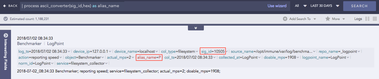
Hexadecimal to ASCII

Syntax:

| process  ascii_converter(fieldname,hex) as string

Example:

| process ascii_converter(sig_id,hex) as alias_name

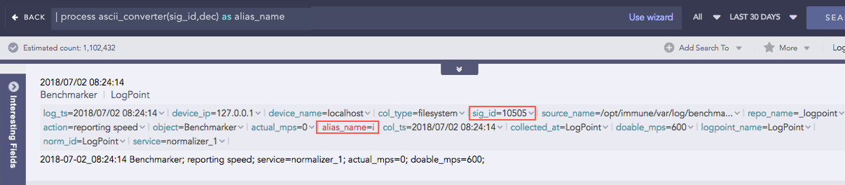
Decimal to ASCII

Syntax:

| process  ascii_converter(fieldname,dec) as string

Example:

| process ascii_converter(sig_id,dec) as alias_name

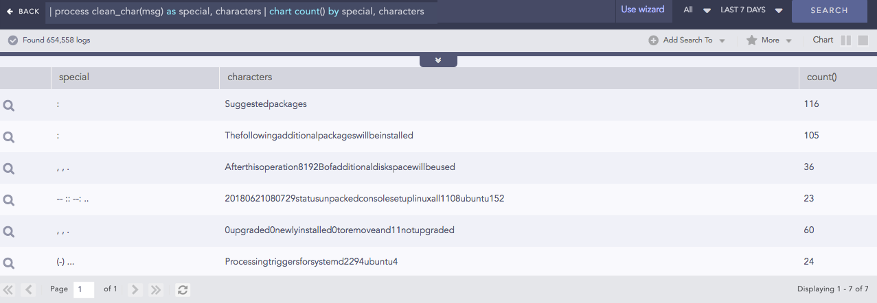
Clean Char¶

Removes all the alphanumeric characters present in a field-value.

Syntax:

| process clean_char(<field_name>) as <string_1>, <string_2>

Example:

| process clean_char(msg) as special, characters
| chart count() by special, characters

Codec¶

Codec is a compression technology with an encoder to compress the files and a decoder to decompress. This process command encodes the field values to ASCII characters or decodes the ASCII characters to their text value using the Base64 encoding/decoding method. Base64 encoding converts binary data into text format so a user can securely handle it over a communication channel.

Syntax:

| process codec(<encode/decode function>, <field to be encoded/decoded>) as <attribute_name>

Example:

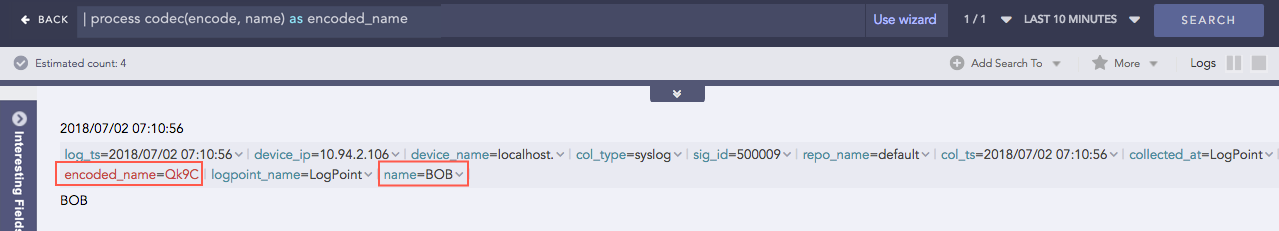
| process codec(encode, name) as encoded_name

Here, the “| process codec(encode, name) as encoded_name” query encodes the value of name field by applying encode function and displays encoded value in encoded_name.

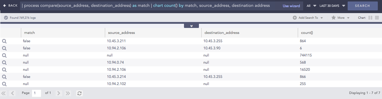
Compare¶

Compares two values to check if they match or not.

Syntax:

| process compare(fieldname1,fieldname2) as string

Example:

| process compare(source_address, destination_address) as match
| chart count() by match, source_address, destination address

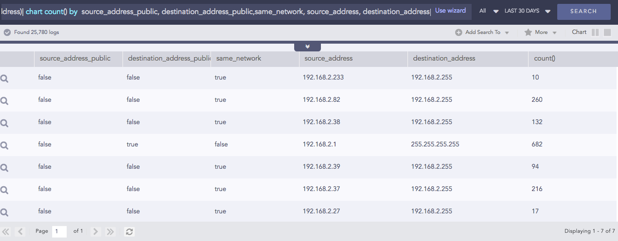
Compare Network¶

Takes a list of IP addresses as inputs and checks if they are from the same network or different ones. It also checks whether the networks are public or private. The comparison is carried out using either the default or the customized CIDR values.

Syntax:

| process compare_network(fieldname1,fieldname2)

Example: (Using default CIDR value)

source_address=* destination_address=*
| process compare_network (source_address, destination_address)
| chart count() by  source_address_public, destination_address_public,
same_network, source_address, destination_address

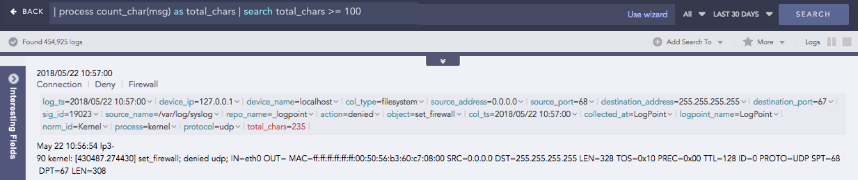
Count Char¶

Counts the number of characters present in a field-value.

Syntax:

| process count_char(fieldname) as int

Example:

| process count_char(msg) as total_chars
| search total_chars >= 100

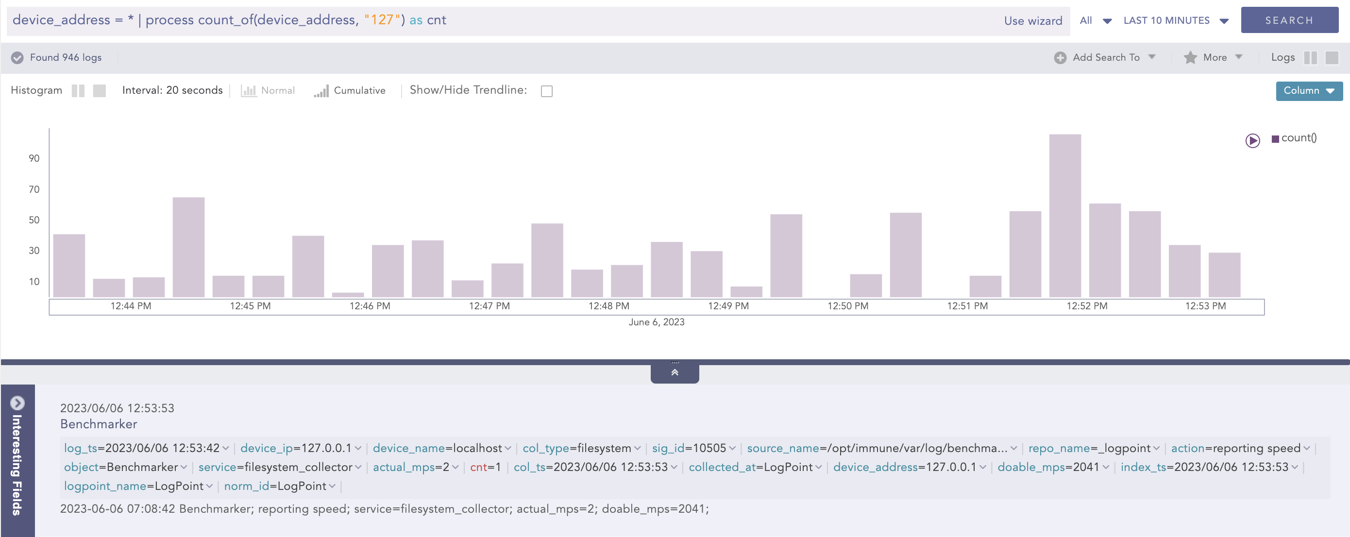
CountOf¶

Takes a field as a parameter and counts the number of times the element(s) occurred in the field’s value.

Syntax:

| process count_of (source field name, string, kind)

Here, the source and search parameters are required.

Example:

| process count_of (device_address, "127") as cnt

Here, the query counts the occurrences of the 127 string in the device_address field value and displays it in cnt.

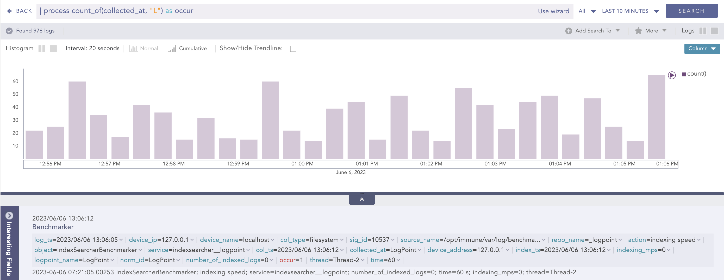
Example:

| process count_of (collected_at, "L") as occur

Here, the query counts the occurrences of L string in the value of collected_at field and displays it in occur.

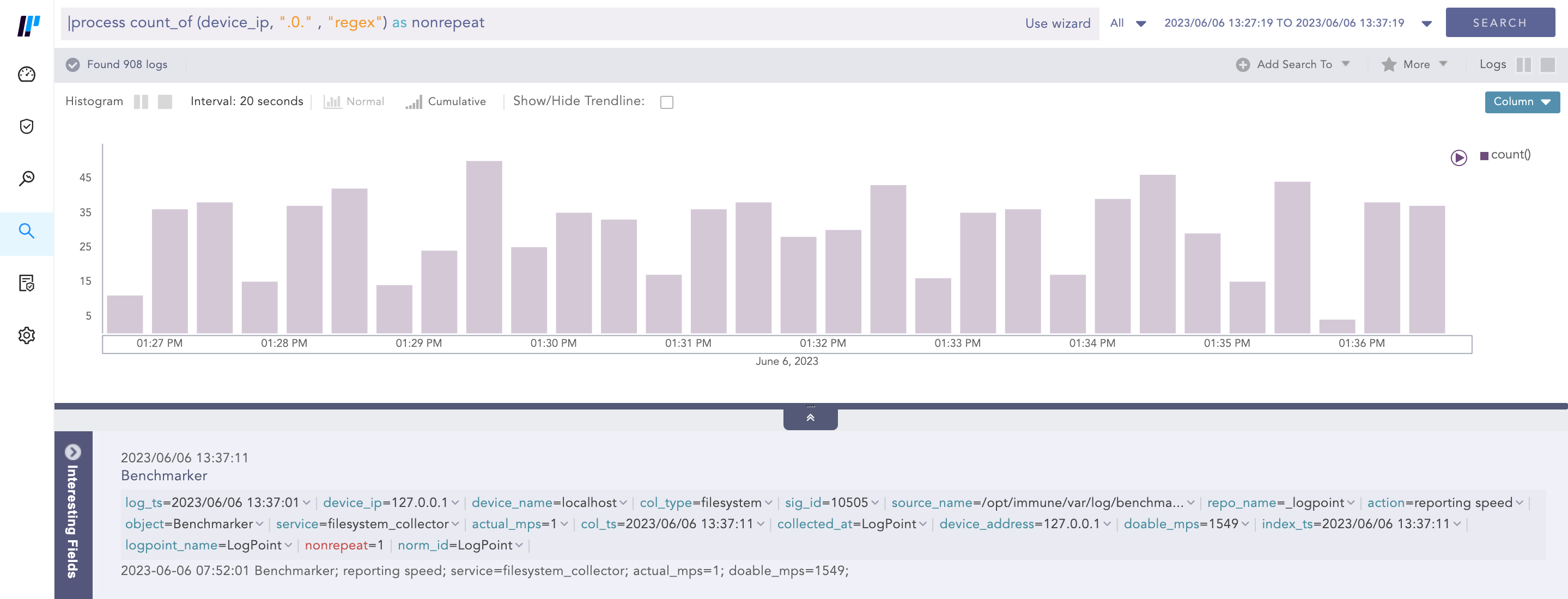
Example:

|process count_of (device_ip, ".0." , "regex") as nonrepeat

Here, the query counts the occcurance of .0. string by applying regex pattern in the value of device_ip field and displays it in nonrepeat.

Current Time¶

Gets the current time from the user and adds it as a new field to all the logs. This information can be used to compare, compute, and operate the timestamp fields in the log message.

Syntax:

| process current_time(a) as string

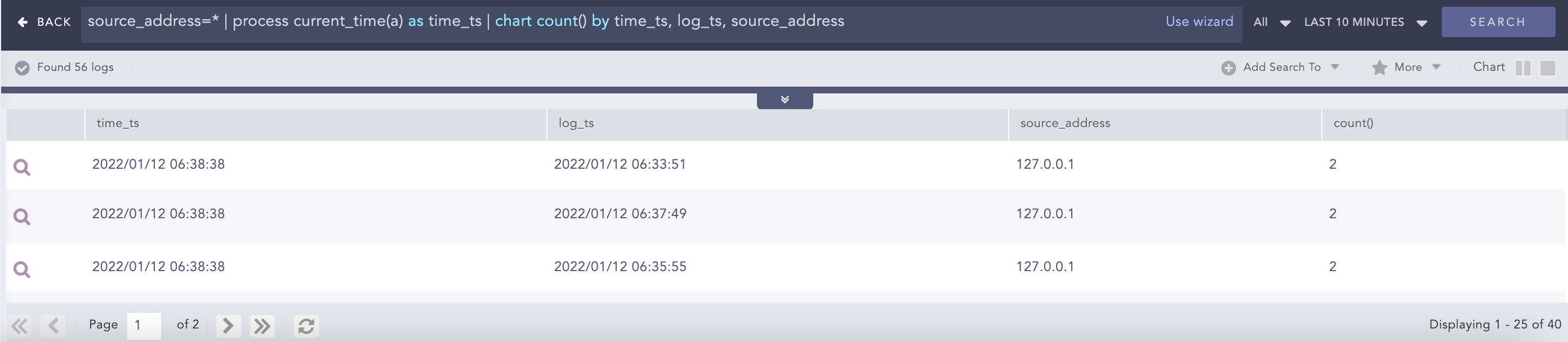
Example:

source_address=* | process current_time(a) as time_ts
| chart count() by time_ts, log_ts, source_address

DatetimeDiff¶

Processes two lists, calculates the difference between them, and returns the absolute value of the difference as the delta. The two lists must contain timestamps. It requires two first and second input parameters that are mandatory and can either be a list or a single field. The third parameter is mandatory and represents the required difference between the two input fields. This difference must be specified in either seconds, minutes or hours. The purpose of the third parameter is to determine how the difference between the two input fields can be represented. For instance, if the difference is specified in seconds, the output will show the absolute difference in seconds.

Syntax:

| process datetime_diff("seconds", ts_list1, ts_list2) as delta

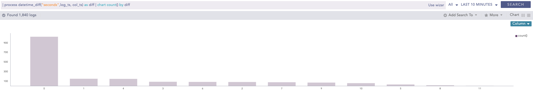
Example:

| process datetime_diff("seconds",log_ts, col_ts) as diff | chart count() by diff

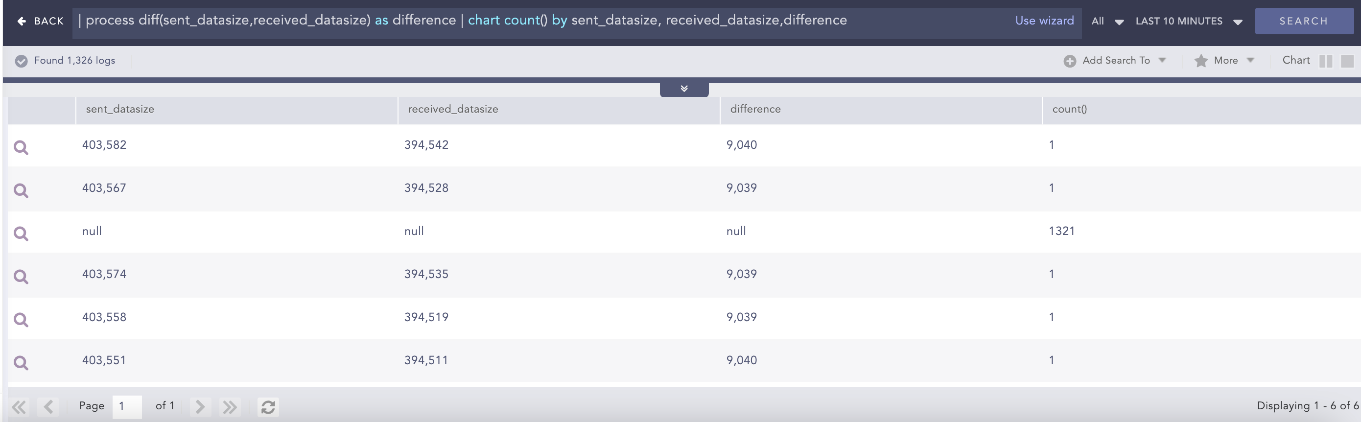
Difference¶

Calculates the difference between two numerical field values of a search.

Syntax:

| process diff(fieldname1,fieldname2) as string

Example:

| process diff(sent_datasize,received_datasize) as difference
| chart count() by sent_datasize, received_datasize,difference

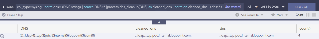
DNS Cleanup¶

Converts a DNS from an unreadable format to a readable format.

Syntax:

| process dns_cleanup(fieldname) as string

Example:

col_type=syslog | norm dns=<DNS.string>| search DNS=*
|process dns_cleanup(DNS) as cleaned_dns
| norm on cleaned_dns .<dns:.*>.
| chart count() by DNS, cleaned_dns, dns

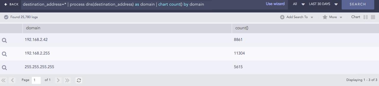
DNS Process¶

Returns the domain name assigned to an IP address and vice-versa. It takes an IP address or a Domain Name and a Field Name as input. The plugin then verifies the value of the field. If the input is an IP Address, it resolves the address to a hostname and if the input is a Domain Name, it resolves the address to an IP Address. The output value is stored in the Field Name provided.

Syntax:

| process dns(IP Address or Hostname)

Example:

destination_address=* | process dns(destination_address) as domain
| chart count() by domain

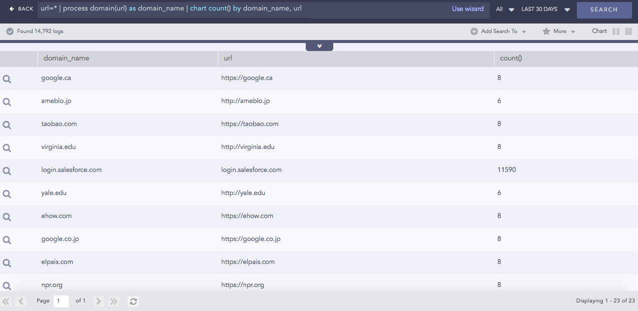
Domain Lookup¶

Provides the domain name from a URL.

Syntax:

| process domain(url) as domain_name

Example:

url=* | process domain(url) as domain_name |
chart count() by domain_name, url

Entropy¶

Entropy measures the degree of randomness in a set of data. This process command calculates the entropy of a field using the Shanon entropy formula and displays data in the provided field. A higher entropy number denotes a data set with more randomness, which increases the probability that a system artificially generated the values and could potentially lead to a malicious conclusion.

Syntax:

| process entropy (field) as field_entropy

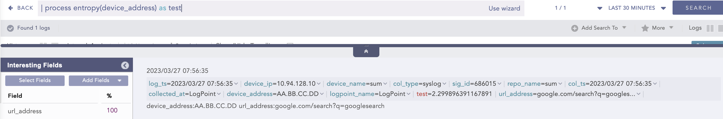
Example:

device_address = *| process entropy (device_address) as test

Here, the “| process entropy (device_address) as test” query calculates the entropy of the device_address field and displays it in test.

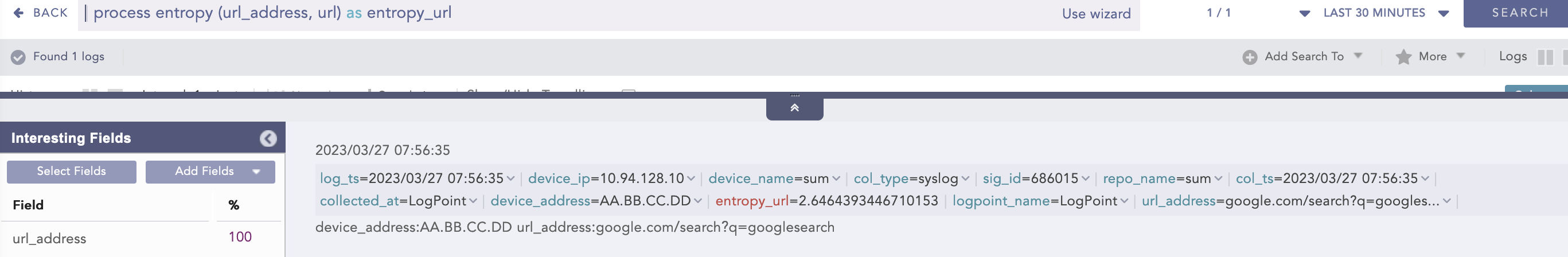
Example:

| process entropy (url_address, url) as entropy_url

Here, the “| process entropy (url_address, url) as entropy_url” query takes url as an optional parameter and extracts the domain name from the url_address to perform entropy calculation on it and displays it in entropy_url.

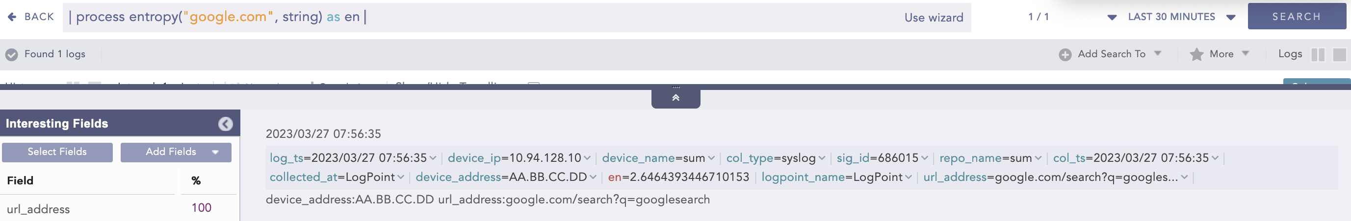
Example:

| process entropy ("google.com", string) as en

Here, the “| process entropy (“google.com”, string) as en” query takes string as an optional parameter and calculates the entropy of google.com raw string field and displays it in en.

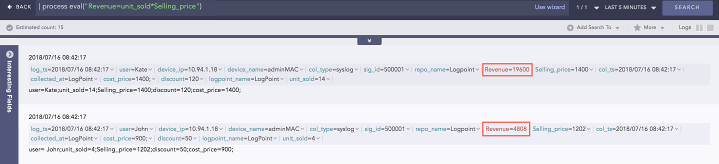
Eval¶

Evaluates mathematical, boolean and string expressions. It places the result of the evaluation in an identifier as a new field.

Syntax:

| process eval("identifier=expression")

Example:

| process eval("Revenue=unit_sold*Selling_price")

Experimental Median Quartile Quantile¶

Performs statistical analysis (median, quartile and quantile) of events based on fields. All these commands take numerical field values as input.

Median

Syntax:

| chart median(fieldname) as string

Example:

doable_mps=* |chart median(doable_mps)

Quartile

Syntax:

| chart quartile(fieldname) as string1, string2, string3

Example:

doable_mps=* |chart quartile(doable_mps)

Quantile

Syntax:

| process quantile(fieldname)

Example:

doable_mps=* | process quantile(doable_mps)
|search quantile>0.99
|chart count() by doable_mps order by doable_mps desc

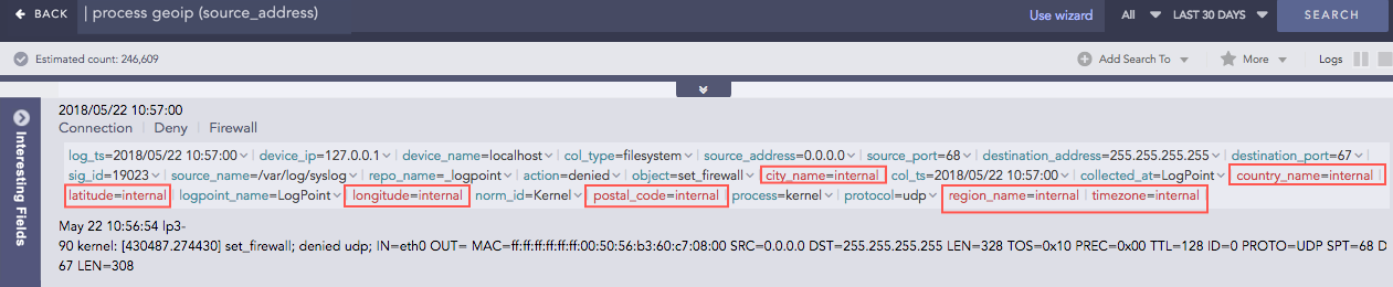
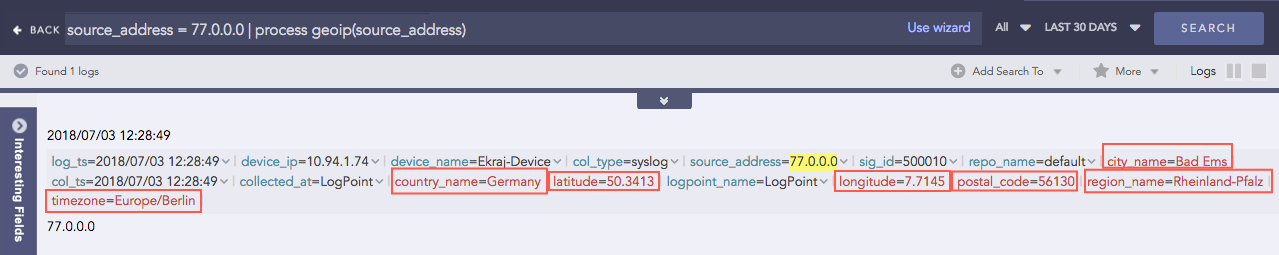
GEOIP¶

Gives the geographical information of a public IP address. It adds a new value “internal” to all the fields generated for the private IP supporting the RFC 1918 Address Allocation for Private Internets.

Syntax:

| process geoip (fieldname)

Example:

| process geoip (source_address)

For the Private IP:

For the Public IP:

Grok¶

Extracts key-value pairs from logs during query runtime using Grok patterns. Grok patterns are the patterns defined using regular expression that match with words, numbers, IP addresses, and other data formats.

Refer to Grok Patterns and find a list of all the Grok patterns and their corresponding regular expressions.

Syntax:

| process grok("<signature>")

A signature can contain one or more Grok patterns.

Example:

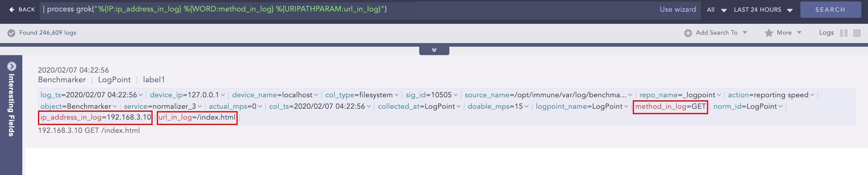
To extract the IP address, method and URL from the log message:

192.168.3.10 GET /index.html

Use the command:

| process grok("%{IP:ip_address_in_log} %{WORD:method_in_log} %{URIPATHPARAM:url_in_log}")

Using this command adds the ip_address_in_log, method_in_log, and url_in_log fields and their respective values to the log if it matches the signature pattern.

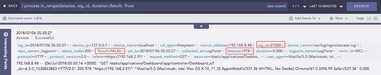
InRange¶

Determines whether a certain field-value falls within the range of two given values. The processed query returns TRUE if the value is in the range.

Syntax:

| process in_range(endpoint1, endpoint2, field, result, inclusion)

where,

endpoint1 and endpoint2 are the endpoint fields for the range,
the field is the fieldname to check whether its value falls within the given range,
result is the user provided field to assign the result (TRUE or FALSE),
inclusion is the parameter to specify whether the range is inclusive or exclusive of
given endpoint values. When this parameter is TRUE, the endpoints will be included for
the query and if it is FALSE, the endpoints will be excluded.

Example:

| process in_range(datasize, sig_id, duration,Result, True)

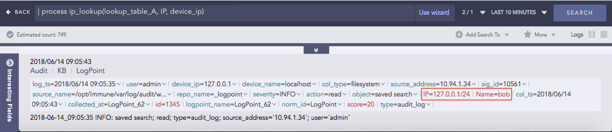
IP Lookup¶

Enriches the log messages with the Classless Inter-Domain Routing (CIDR) address details. A list of CIDRs is uploaded in the CSV format during the configuration of the plugin. For any IP Address type within the log messages, it matches the IP with the content of the user-defined Lookup table and then enriches the search results by adding the CIDR details.

Syntax:

| process ip_lookup(IP_lookup_table, column, fieldname)
 where IP_lookup_table is the lookup table configured in the plugin,
 Column is the column name of the table which is to be matched
  with the fieldname of the log message.

Example:

| process ip_lookup(lookup_table_A, IP, device_ip)

Here, the command compares the IP column of the lookup_table_A with the device_ip field of the log and if matched, the search result is enriched.

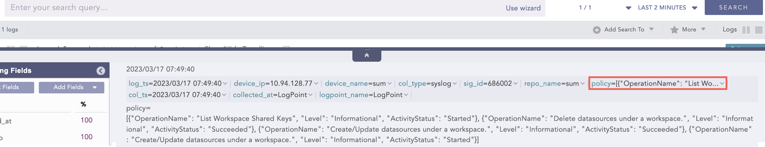
JSON Expand¶

Takes the field with a valid JSON array value and:

1. Splits the array into individual JSON objects.

2. Creates multiple log instances for each array value of that field.

3. Assigns the original field name to each array value.

Syntax:

| process json_expand (field name)

Use Case 1:

For example, a normalized events field with a valid JSON array value.

events = [

{“source_ip”: “192.168.0.1”, “action”: “login”, “status”: “success”},

{“source_ip”: “192.168.0.2”, “action”: “login”, “status”: “failure”},

{“source_ip”: “192.168.0.3”, “action”: “login”, “status”: “success”}

]

Query:

| process json_expand(events)

Output:

Index Log 1:

events = {“source_ip”: “192.168.0.1”, “action”: “login”, “status”: “success”}

Index Log 2:

events = {“source_ip”: “192.168.0.2”, “action”: “login”, “status”: “failure”}

Index Log 3:

events = {“source_ip”: “192.168.0.3”, “action”: “login”, “status”: “success”}

You can further normalize JSON array values (JSON objects) into indexed logs.

Syntax:

| process json_expand (field name, x)

x enables normalizing the key-value pair of JSON array into the indexed logs. The normalization occurs up to two levels, and a JSON field is ignored if it conflicts with the existing normalized field.

Use Case 2:

For example, a normalized evidence field with a valid JSON array value.

evidence = [

{ “odata_type”:”userAccount”, “userAccount”: {“accountName”: “Logpoint”,”azureUserId”: “177”, “details” :{“department”: “IT”, “accountName”: “Logpoint_IT”} } } },

{ “odata_type”:”ipAddress”,”ipAddress”: “192.168.1.1” }

]

Query:

| process json_expand(evidence, x)

Output:

Index Log 1:

evidence = {“odata_type”:”userAccount”, “userAccount”: {“accountName”: “Logpoint”,”azureUserId”: “177”, “details” :{“department”: “IT”, “accountName”: “Logpoint_IT”} } } } // preserving the original field

odata_type = userAccount

userAccount_accountName = Logpoint

userAccount_azureUserId = 177

Here,

• In level 1, odata_type and userAccount fields are extracted, and in level 2, userAccount_accountName and userAccount_azureUserId fields.

• userAccount_details_department and userAccount_details_accountName fields can be extracted manually.

• userAccount_details_accountName field is ignored since userAccount_accountName already exists.

Index Log 2:

evidence = {“odata_type”:”ipAddress”,”ipAddress”:”192.168.1.1”} // preserving the original field

odata_type = ipAddress

ipAddress = 192.169.1.1

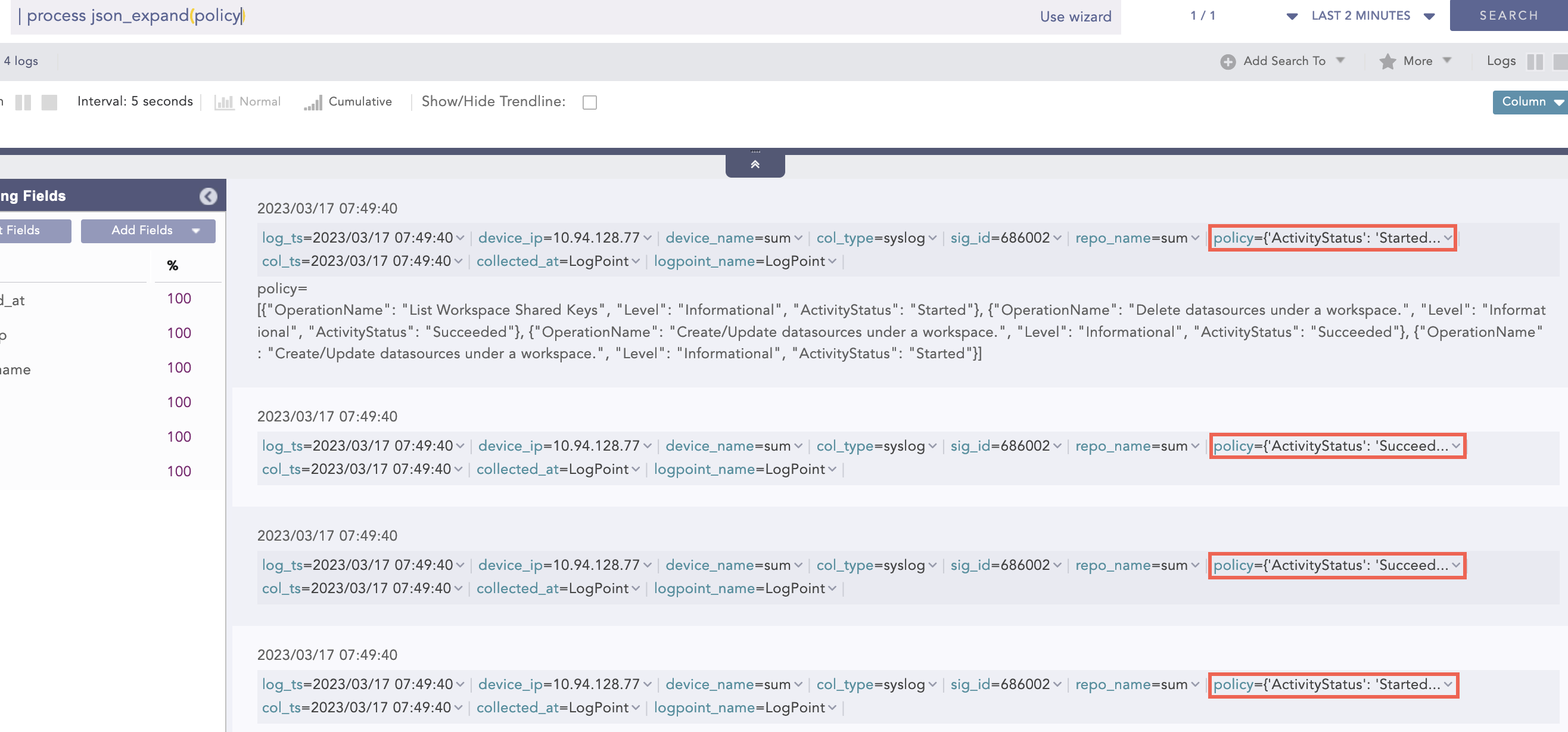
Example:

| process json_expand (policy)

The log before applying the JSON Expand query¶

Four log instances after applying the JSON Expand query¶

Here, the “| process json_expand (policy)” query expands the policy field into four log instances. After expansion, each array value takes the policy as a field name.

JSON Parser¶

The JavaScript Object Notation (JSON) Parser reads JSON data and extract key values from valid JSON fields of normalized logs. A string filter is applied to the provided field, which defines a path for extracting values from it. The filter contains a key, which can be alphanumeric and special characters except square brackets ([]), backtick (`) and tilde (~). These exceptional characters are reserved for essential use cases, such as mapping the list and selecting a condition in JSON Parser.

Syntax:

| process json_parser (field name, "filter") as field name

The supported filter formats are:

1. Chaining for nested JSON

   Example: .fields.user.Username

2. Array access

   Example: .[1]

The supported filters are:

1. flatten

   It collapses nested arrays into a single, flat array and simplifies the structure of deeply nested arrays by combining all their items into a single level.

   Example:

   arr = [“John”, “Doe”, [“Hello”, “World”], “Welcome”]

   Query:

   process json_parser(arr, “flatten”) as flattened_arr

   Output:

   flattened_arr = [“John”, “Doe”, “Hello”, “World”, “Welcome”]

2. reverse

   It reverses the order of items in an array, simplifying actions where the order of items needs to be inverted, such as sorting or searching.

   Example:

   jsn_list = {“severity”: [5,4,1,8]}

   Query:

   process json_parser(jsn_list, “.severity | reverse”) as reversed_severity

   Output:

   reversed_severity = [8, 1, 4, 5]

   

   Using Reverse Filter with Flatten and Sort Filters¶

3. sort

   It arranges the items of an array in ascending order.

   The items of an array are sorted in the following order:

   1. null

   2. false

   3. true

   4. numbers

   5. strings, lexicographically

   6. objects

   Example 1:

   jsn_list = {“severity”: [5,4,1,8]}

   Query:

   process json_parser(jsn_list, “.severity | sort”) as sorted_severity

   Output:

   sorted_severity = [1, 4, 5, 8]

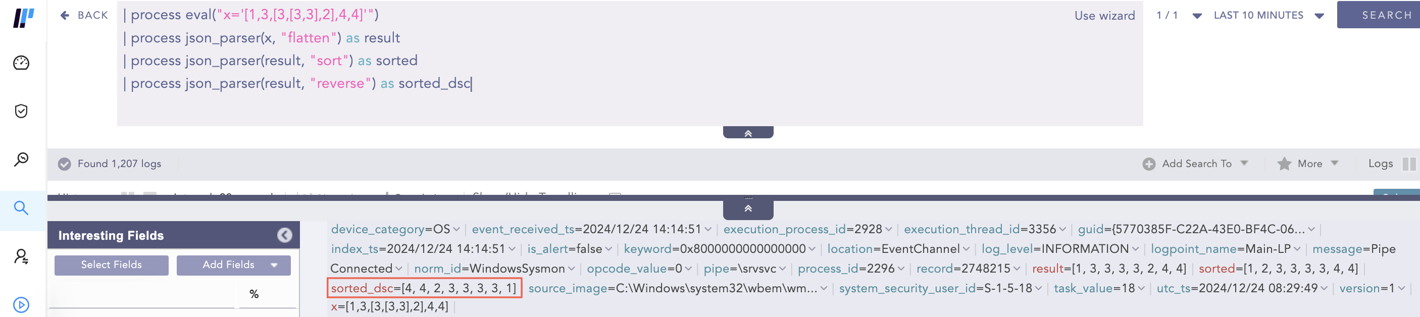
   Example 2:

   x: [true, false, null, “abc”, “ab”, 0, 5, 1]

   Query:

   process eval (“x=’[true, false, null, “abc”, “ab”, 0, 5, 1]’”)

   process json_parser(x, “sort”) as sorted_result

   Output:

   sorted_result = [null, false, true, 0, 1, 5, “ab”, “abc”]

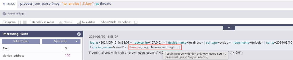
4. to_entries

   It transforms a JSON object into an array of object, where each key-value pair becomes an object with key and value fields. This helps process key-value pairs or convert an object into a more manageable structure in a query result.

   Example:

   jsn_obj = {“name”: “John Doe”, “age”: 30, “email”: “john@example.com”}

   Query:

   process json_parser(jsn_obj, “to_entries”) as key_fields

   Output:

   key_fields = [ {“key”: “name”,”value”: “John Doe”}, {“key”: “age”,”value”: 30}, {“key”: “email”,”value”: “john@example.com”} ]

   

   Using to_entries Filter to get Key Fields¶

5. unique

   It removes duplicate items from an array. After applying the filter, the resulting array contains only one instance of each unique item from the original array, ensuring that all values in the returned array are distinct.

   Example:

   jsn_list = {“files”: [“1.exe”, “1.exe”, “2.exe”]}

   Query:

   process json_parser(jsn_list, “.files | unique”) as unique_file

   Output:

   unique_file = [“1.exe”, “2.exe”]

JSON Parser supports map and select functions for applying filters with true conditional statements. The supported conditional operators are: =, !=, >, < , >= and <=.

General syntax to use map and select functions:

| process json_parser(field name, ".[condition]") as field name

JSON Parser converts a non-JSON value to a list with a single item when dot (.) filter is applied.

Use Case:

For example, a normalized col_type field with a non-JSON filesystem value.

Query:

| process json_parser(col_type, ".") as result

Output:

result=['filesystem']

JSON Parser supports negative indexes, enabling the return of the last element of a data set.

Use Case:

For example, a normalized ip field appearing as multiple value array.

ip = [10,20,30,40]

Query:

| process json_parser(ip, ".[-1]") as last_item

Output:

last_item = 40

Example 1:

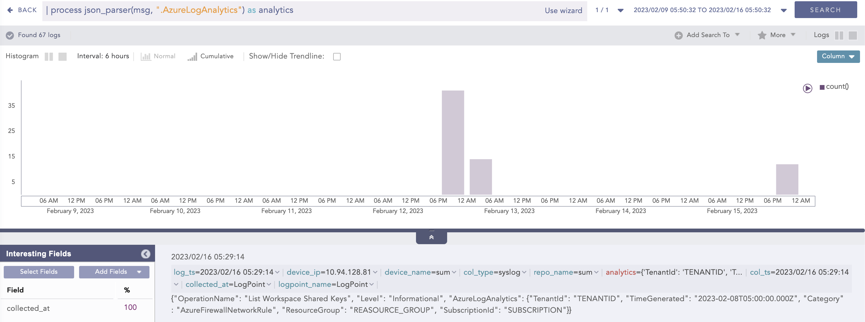
| process json_parser (msg, ".AzureLogAnalytics") as analytics

Here, the “| process json_parser (msg, “.AzureLogAnalytics”) as analytics” query applies the AzureLogAnalytics filter to the msg field and extracts the key values to the analytics field.

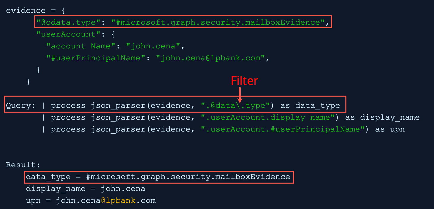
Example 2:

In filter, the backslash escaped the period before type and query applies the filter to the evidence field and extracts the key value to the data_type field.

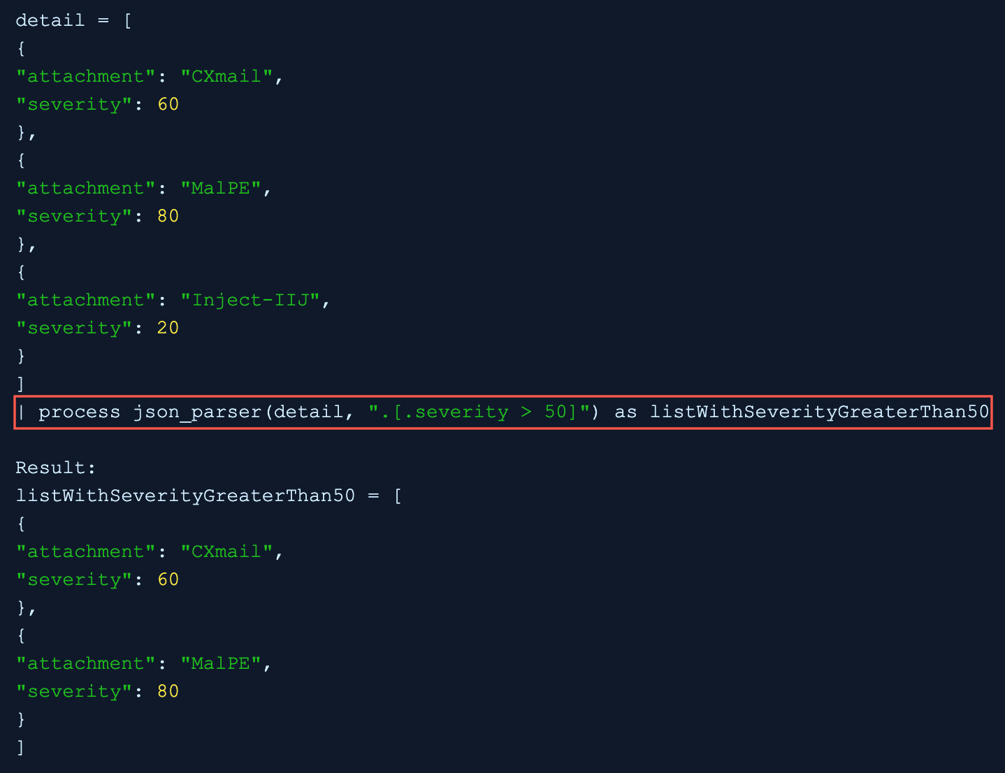
Example 3:

In the .[.severity>50] filter, a conditional statement severity>50 is used and the “| process json_parser(detail, “.[.severity > 50]”) as listWithSeverityGreaterThan50” query applies the filter to the detail field and extracts the list of key values with the true condition to the listWithSeverityGreaterThan50 field.

ListLength¶

For an indexed field with a list of values, such as destination_port = [67, 23, 45, 12, 10], the command returns the number of elements in the list.

Syntax:

| process list_length(list) as field name

Use Case:

For example, an indexed usernames field appearing as multiple value array.

usernames = [‘Alice’, ‘Bob’, ‘Carol’, ‘John’]

Query:

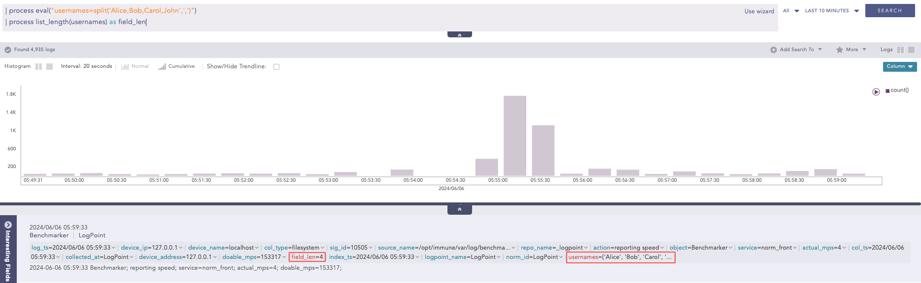
| process eval("usernames=split('Alice,Bob,Carol,John',',')") | process list_length(usernames) as field_len

Output:

4

Here, the “| process eval(“usernames=split(‘Alice,Bob,Carol,John’,’,’)”)” query splits the string ‘Alice,Bob,Carol,John’ into a list of strings and assigns the list to usernames field. Then, the “| process list_length(usernames) as field_len” query calculates the length of the usernames field values and returns the result in the field_len field.

Example:

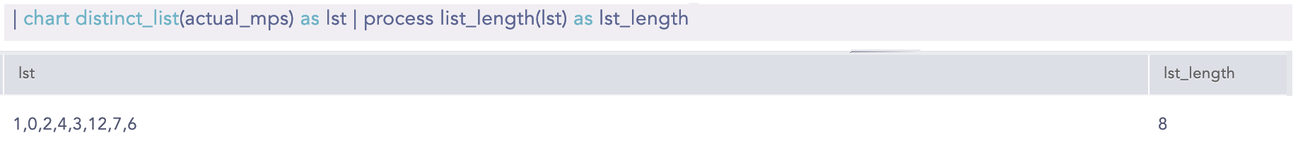
| chart distinct_list(actual_mps) as lst | process list_length(lst) as lst_length

Here, the “| chart distinct_list(actual_mps) as lst” query creates a distinct list of values from the actual_mps field and assigns it to the lst field. Then, the “| process list_length(lst) as lst_length” query calculates the length of the lst field values and returns the result in the lst_length field.

ListPercentile¶

Calculates the percentile value of a given list. It requires at least two input parameters. The first parameter is mandatory and must be a list. This command can also accept up to five additional parameters. The second parameter must be an alias, which is used in conjunction with the percentile percentage to determine the required percentile. The alias is concatenated with the percentile percentage to store the required percentile value.

Syntax:

| process list_percentile(list, 25, 75, 95, 99) as x

Result: x_25th_percentile = respective_value
    x_75th_percentile = respective_value
    x_95th_percentile = respective_value
    x_99th_percentile = respective_value

General:
| process list_percentile(list,p) as aliasalias_pth_percentile

Example:

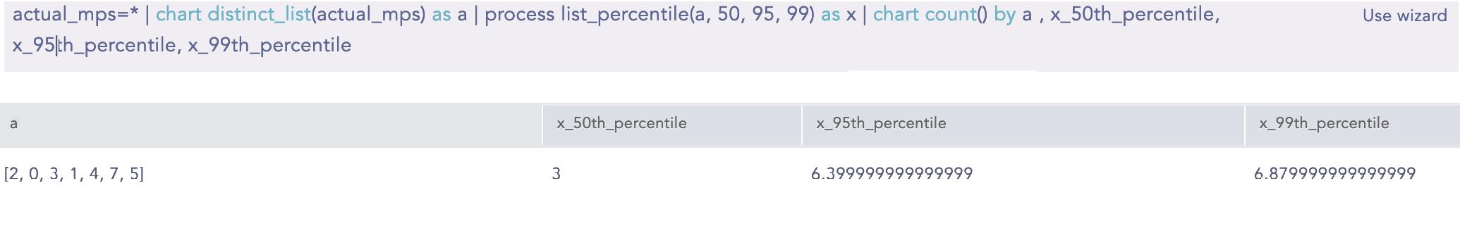
| actual_mps=* chart distinct_list(actual mps) as a | process list_percentile(a, 50, 95,99) as x | chart count() by a,
x_50th_percentile, x_95th_percentile, x_99th_percentile

Next¶

Takes a list and an offset as input parameters and returns a new list where the elements of the original list are shifted to the left by the specified offset. The maximum allowable value for the offset is 1024. For example, if the original list is [1, 2, 3, 4, 5, 6] and the offset is 1, the resulting list would be [2, 3, 4, 5, 6]. Similarly, if the offset is 2, the resulting list would be [3, 4, 5, 6]. This command requires two parameters as input. The first is mandatory and must be a list. The second parameter is mandatory and represents the offset value. An alias of 1 must be provided as input.

Syntax:

| process next(list, 1) as next_list|  process next(list, 2) as next_list_2

Example:

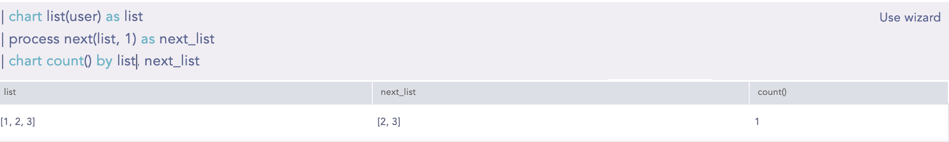
| chart list(user) as list | process next(list, 1) as next_list | chart count() by list next_list

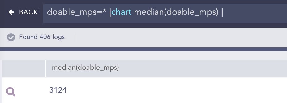
Percentile¶

Percentiles are numbers below which a portion of data is found. This process command calculates the statistical percentile from the provided field and informs whether the field’s value is high, medium or low compared to the rest of the data set.

Syntax:

| chart percentile (field name, percentage)

Example:

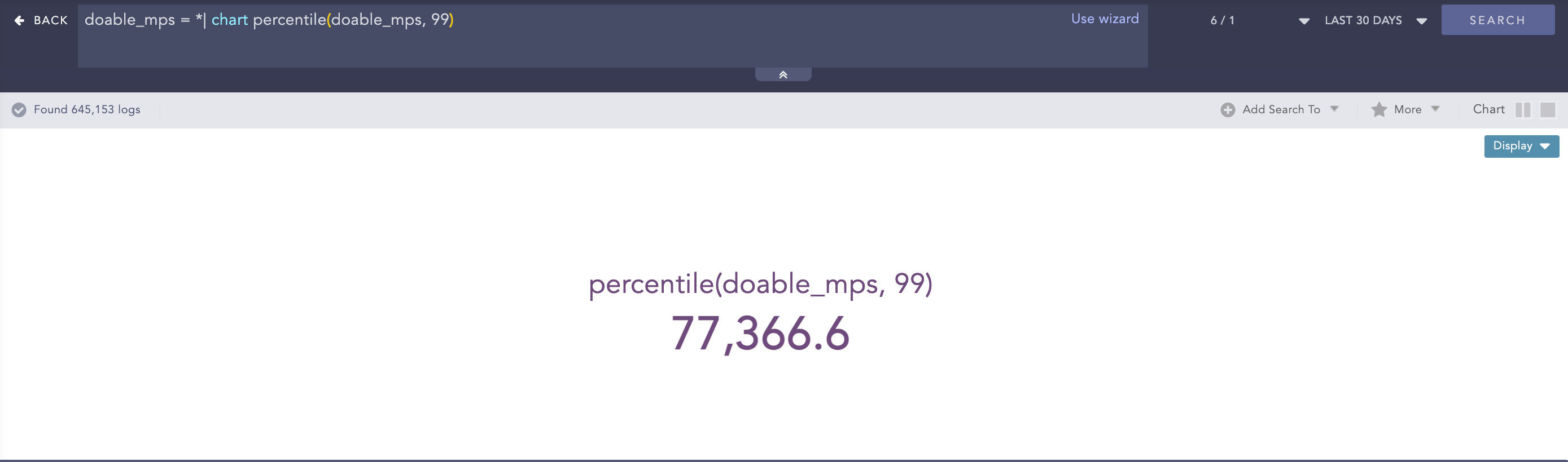
doable_mps = *| chart percentile (doable_mps, 99)

Here, the “| chart percentile (doable_mps, 99)” command calculates the percentile for the value of the doable_mps field.

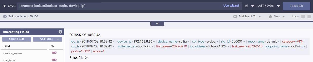
Process lookup¶

Looks up related data from a user defined table.

Syntax:

| process lookup(table,field)

Example:

| process lookup(lookup_table, device_ip)

Regex¶

Extracts specific parts of the log messages into custom field names based on a regex pattern applied.

Syntax:

| process regex("_regexpattern", _fieldname)
| process regex("_regexpattern", "_fieldname")

Both syntaxes are valid.

You can add a filter parameter in the syntax with true or false values to apply a filter to the extracted value. The filter allows only the values matching the regex pattern to be included in the output.

If the filter value is true, the filter is applied to the extracted values and the regex command output matches only those values. If the value is false, the filter is not applied, and the output includes matched and non-matched values.

If a filter is not specified, the default value is false.

Syntax:

| process regex("_regexpattern", _fieldname, "filter = true")

Use Case 1:

For example, in the indexed log below,

Log Entry:

1. user=John Smith, log_id=log_1
2. user=Ketty Perry, log_id=log_2
3. user=Keth Vendict, log_id=log_3
4. user=Keegan Pele, log_id=log_4

Query:

| process regex("(?P<fst_name>Ket\S+)", user, "filter=true")

Regex pattern:

In (?P<fst_name>KetS+),

• (?) indicates the start of a capture group. A capture group is a way to define and extract specific parts of a text or pattern in a regular expression. It’s like putting parentheses around the part of the text you want to focus on.

• P indicates literal character.

• <fst_name> is the field name assigned to the capture group. It is the custom field name.

• Ket matches the literal characters Ket.

• S+ matches one or more non-whitespace characters after Ket in the log.

Process:

• The regex pattern searches for sequences that start with Ket followed by non-whitespace characters in each log’s user field.

• The pattern matches Ketty and Keth from log entries 2 and 3.

• The pattern captures the matched values, and the filter is applied before assigning the values to the fst_name field.

Output:

1. user=Ketty Perry, log_id=log_2, fst_name=Ketty
2. user=Keth Vendict, log_id=log_3, fst_name=Keth

These are the first names extracted from the user field where the user’s name starts with Ket.

Use Case 2:

For the same log entries above,

Query:

| process regex("(?P<fst_name>Ket\S+)", user, "filter=false")

or

When the filter value is false or the filter is not specified, the pattern captures the matched values. It assigns matched and non-matched user field values to the fst_name field.

Output:

1. user=John Smith, log_id=log_1
2. user=Ketty Perry, log_id=log_2, fst_name=Ketty
3. user=Keth Vendict, log_id=log_3, fst_name=Keth
4. user=Keegan Pele, log_id=log_4

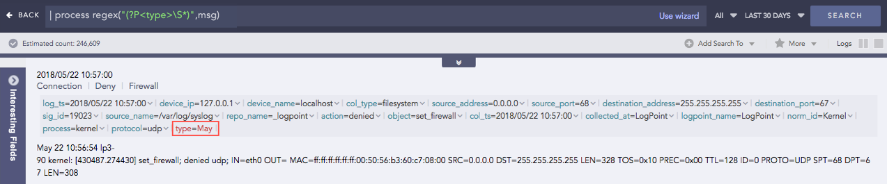
Example 1:

| process regex("(?P<type>\S*)",msg)

Here, the “| process regex(“(?P<type>S*)”,msg)” query extracts any sequence of non-whitespace characters from the msg field and assigns it to a capture grouped type field.

(?P<type>S*) is the regular expression pattern where,

• (?P<type>…) is a capture group, marked by (?P<…>). It assigns the type filed name to the matched pattern.

• S matches zero or more non-whitespace characters.

• ‘*’ specifies the zero or more occurrences of non-whitespace characters.

• msg is the data field to which the regular expression will be applied.

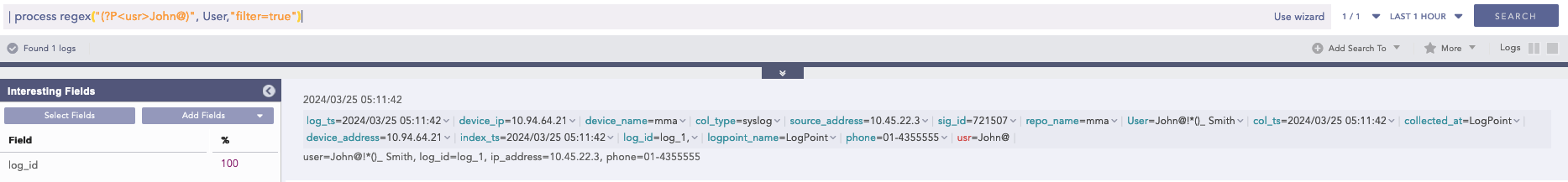
Example 2:

| process regex("(?P<usr>John@)", User,"filter=true")

Here, the “| process regex(“(?P<usr>John@)”, User,”filter=true”)” query captures the text in the User field that matches the John@ pattern and assigns it to the captured grouped usr field.

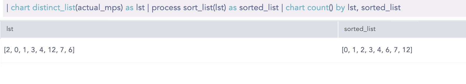
SortList¶

Sorts a list in ascending or descending order. By default, the command sorts a list in ascending order. The first parameter is mandatory and must be a list. The second parameter desc is optional.

Syntax:

| process sort_list(list) as sorted_list
| process sort_list(list, "desc") as sorted_list

Example:

chart distinct list(actual_mps) as lst | process sort_list(lst) as LP_KB_Dynamictable_Populate_Values | chart count by lst, sorted list

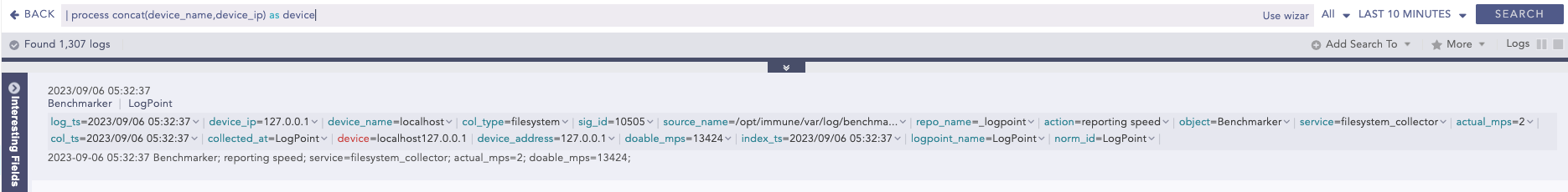
String Concat¶

Joins multiple field values of the search results.

Syntax:

| process concat(fieldname1, fieldname2, ...., fieldnameN) as string

Example:

| process concat(device_name,device_ip) as device

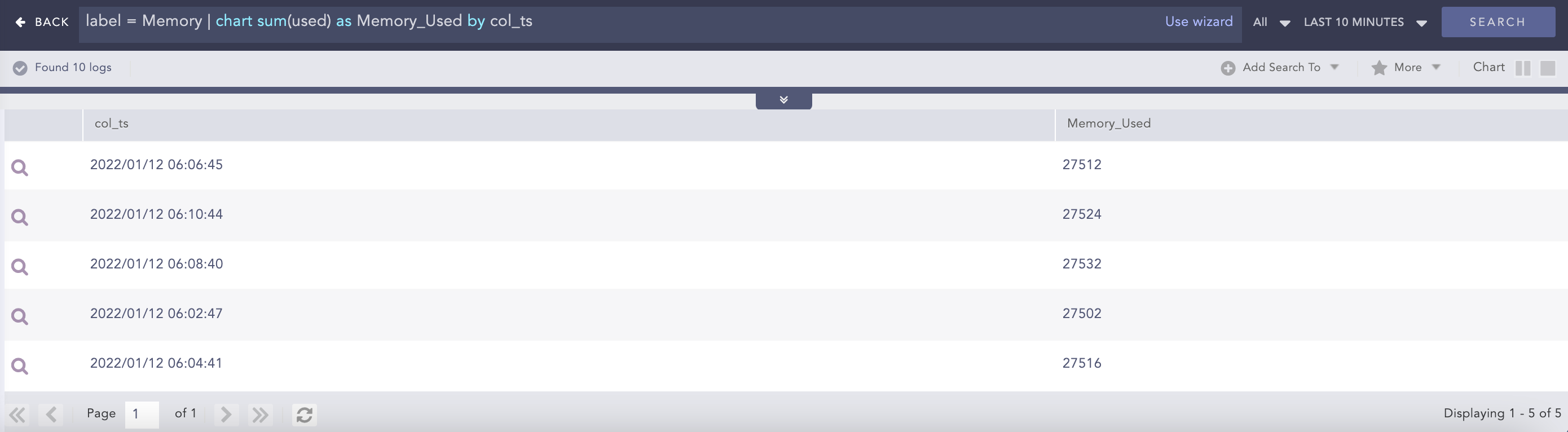
Summation¶

Calculates the sum between two numerical field values of a search.

Syntax:

| chart sum(fieldname)

Example:

label = Memory | chart sum(used) as Memory_Used by col_ts

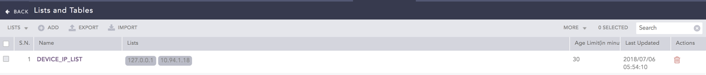
toList¶

Populates the dynamic list with the field values of the search result. To learn more, go to Dynamic List.

Syntax:

| process toList (list_name, field_name)

Example:

device_ip=* | process toList(device_ip_list, device_ip)

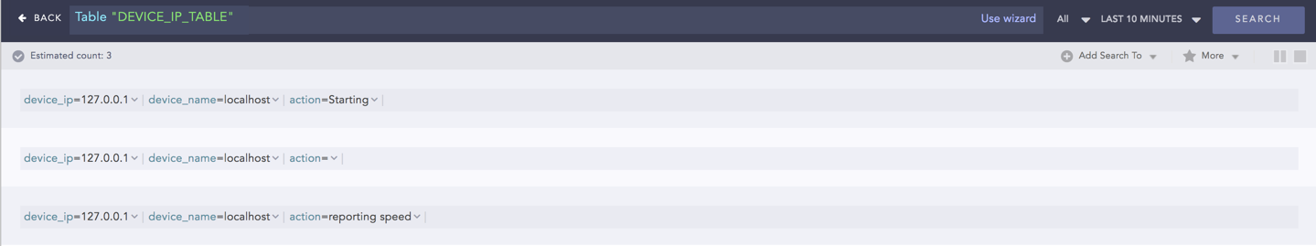
toTable¶

Populates the dynamic table with the fields and field values of the search result. To learn more, go to Dynamic Table.

Syntax:

| process toTable (table_name, field_name1, field_name2,...., field_name9)

Example:

device_ip=* | process toTable(device_ip_table, device_name, device_ip, action)

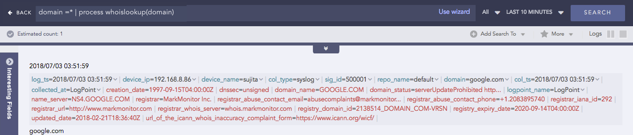
WhoIsLookup¶

Enriches the search result with the information related to the given field name from the WHOIS database.The WHOIS database consists of information about the registered users of an Internet resource such as registrar, IP address, registry expiry date, updated date, name server information and other information. If the specified field name and its corresponding value are matched with the equivalent field values of the WHOIS database, the process command enriches the search result, however, note that the extracted values are not saved.

Syntax:

| process whoislookup(field_name)

Example:

| chart distinct_list(log_ts) as log_ts_list, distinct_list(col_ts) as col_ts_list
| process datetime_diff("seconds", log_ts_list, col_ts_list) as delta
| chart count() by log_ts_list, col_ts_list, delta`

    domain =* | process whoislookup(domain)